
Understanding Absolute and Incremental Compensation
Learning to manipulate absolute and incremental CNC compensation can not only extend the life of a given machine but also ultimately result in improved manufacturing flexibility, accuracy, and quality.
Share


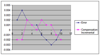
Graph of the error versus the incremental compensation.
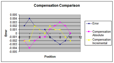
Graph comparing absolute and incremental compensation.
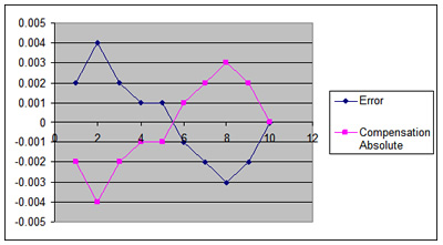
Graph of the error versus the absolute compensation.
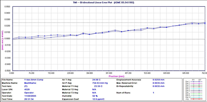
Bi-directional Linear Error Plot
Introduction
In today’s manufacturing environment, it is more and more commonplace to utilize laser measurement systems for the calibration of CNC machines. After all, companies routinely calibrate the gages they use for verifying dimensional information so why not go ahead and do the same for the equipment that create the dimensions? The benefits of a preventive maintenance program that includes the calibration of CNC machines are many. Reduced scrap, reduced rework at the detail and assembly level, and increased shop floor flexibility are just a few. Add to this the ability to know if a machine is adequate to manufacture a given part before putting it on the machine (or getting the work) and it all adds up to give you significant insight into the manufacturing capabilities of an organization.
However, there is a problem with the process. Today’s shops have a myriad of machines with many different types of controls that have different capabilities, communication methods, and varying approaches to compensation. These variables combined with today’s leaner and meaner maintenance organizations present quite a challenge to those who need to utilize the electronic compensation inherent in the controls. Maintenance groups across the country (and world) struggle with the issue of compensation.


Not too long ago, I was working for a rather well known laser manufacturer and had the unique opportunity to travel all throughout North America talking to end users of the equipment. By and large, the most common question was, well the laser is great, but, "How do you comp this machine?" The more I traveled, the more I heard the same question. I even had conversations with machine tool control manufacturers of many varieties and explained to them that the great compensation they were making available in their controls was fantastic but that unfortunately, nobody knew how to take advantage of it – it just wasn’t clear.
In this article, we will seek to get some foundational theory underneath the various types of compensation and further attempt to give examples of its formulation. For simplicity sake, we will focus on linear compensation. Future articles will begin to deal with aspects of straightness and squareness compensation. Ultimately, we will touch on the aspects of volumetric compensation. However, first things first: let’s start with linear.
Background
Before we dive in, please let me say that it is not my intent to endorse any specific type of compensation in this series of article or further more any brand of control. As will become clear in future articles (and most of you likely already know this), they all have their strengths.
There are two basic types of compensation available in today’s controls: Absolute and Incremental. Incremental compensation is typically found in Japanese controls and Absolute compensation is found in most others. As the details of these types of compensation are investigated, it may be seen that there are advantages in each of the approaches.
Absolute Compensation
With absolute compensation, individual points stand alone. For the most part, the value entered into the control is the opposite value of the error observed, however, this depends on the control. Consider the error profile depicted below where the first column represents the measured point and the second column the measured error. This is typical of the linear data obtained from a laser measurement system:
Point Error
1 0.002
2 0.004
3 0.002
4 0.001
5 0.001
6 -0.001
7 -0.002
8 -0.003
9 -0.002
10 0
The resulting compensation for an absolute control is then:
Point Error Compensation
1 0.002 -0.002
2 0.004 -0.004
3 0.002 -0.002
4 0.001 -0.001
5 0.001 -0.001
6 -0.001 0.001
7 -0.002 0.002
8 -0.003 0.003
9 -0.002 0.002
10 0 0
Based on the absolute model, it should then be expected that the graphs of the error versus the compensation to show an inversion from one another as shown below:
Incremental Compensation
Basically, incremental compensation operates under the premise that each point influences the other. That is to say, changes in a previous point (from a given point) will influence all points from there on to the end of the string. While initially this may seem somewhat cumbersome, it can be quite useful. In situations where some relatively modest scaling may be seen, the modification of the first compensation value will be felt through the entire curve.
When working with incremental compensation, the values are additive from one point to another. Going back to the same error profile mentioned in the discussion of the absolute compensation model, the differences may be seen. Again, the first column represents the point number with the second column representing the associated error as measured by a laser.
Point Error
1 0.002
2 0.004
3 0.002
4 0.001
5 0.001
6 -0.001
7 -0.002
8 -0.003
9 -0.002
10 0
The first point would be -.002 (to get to zero), the second, another -.002, the third, .002 and so on. Note here that the compensation value is the change from one point to another as opposed to the absolute value as explained earlier in the absolute compensation discussion. The final compensation table would then look like:
Point Error Compensation
1 0.002 -0.002
2 0.004 -0.002
3 0.002 0.002
4 0.001 0.001
5 0.001 0
6 -0.001 0.002
7 -0.002 0.001
8 -0.003 0.001
9 -0.002 -0.001
10 0 -0.002
To compare the two methods simultaneously, please see the graph shown below. This shows the overall error, the absolute compensation, and the incremental compensation graphs overlaid.
Exercises
A sample set of exercises has been included (along with answers) with this article so that this may be practiced.
Summary
Certainly it is said by many users of controls, laser, and associated software that the absolute compensation method makes more intuitive sense. As mentioned before, this type of compensation is seen on mostly non-Japanese controls however the reality is that, once understood, both compensation approaches offer unique abilities. Either way, with today’s shops, one is bound to find both types of controls. Learning to manipulate both types of compensation can not only extend the life of a given machine but also ultimately result in improved manufacturing flexibility, accuracy, and quality.
Sample Exercises
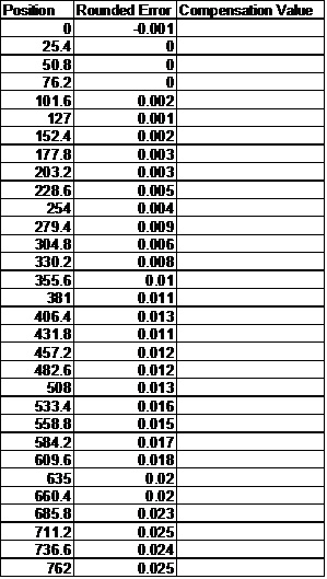
The graph below formulates compensation values based upon both incremental and absolute controls. Note the dimensional data is given in millimeters.
The Raw Data:
Position Forward Error
0 -0.000991
25.4 0.000103
50.8 0.000484
76.2 0.000151
101.6 0.002265
127 0.00063
152.4 0.001902
177.8 0.002967
203.2 0.003343
228.6 0.00499
254 0.004481
279.4 0.008745
304.8 0.00625
330.2 0.008284
355.6 0.00981
381 0.011361
406.4 0.013371
431.8 0.011046
457.2 0.012257
482.6 0.012499
508 0.012693
533.4 0.015842
558.8 0.015212
584.2 0.017441
609.6 0.017538
635 0.019621
660.4 0.020493
685.8 0.022915
711.2 0.024853
736.6 0.023836
762 0.02495
To begin your exercise, fill in the compensation values. For convenience, values have been rounded to the nearest micron. First, assume an incremental compensation approach.
The answers may be seen below:
Position Rounded Error Compensation Value
0 -0.001 0.001
25.4 0 -0.001
50.8 0 0
76.2 0 0
101.6 0.002 -0.002
127 0.001 0.001
152.4 0.002 -0.001
177.8 0.003 -0.001
203.2 0.003 0
228.6 0.005 -0.002
254 0.004 0.001
279.4 0.009 -0.005
304.8 0.006 0.003
330.2 0.008 -0.002
355.6 0.01 -0.002
381 0.011 -0.001
406.4 0.013 -0.002
431.8 0.011 0.002
457.2 0.012 -0.001
482.6 0.012 0
508 0.013 -0.001
533.4 0.016 -0.003
558.8 0.015 0.001
584.2 0.017 -0.002
609.6 0.018 -0.001
635 0.02 -0.002
660.4 0.02 0
685.8 0.023 -0.003
711.2 0.025 -0.002
736.6 0.024 0.001
762 0.025 -0.001
Next, look at the same data in absolute terms. Fill in your data in the following chart:
In absolute terms, the compensation then looks as follows:
Position Rounded Error Compensation Value
0 -0.001 0.001
25.4 0 0
50.8 0 0
76.2 0 0
101.6 0.002 -0.002
127 0.001 -0.001
152.4 0.002 -0.002
177.8 0.003 -0.003
203.2 0.003 -0.003
228.6 0.005 -0.005
254 0.004 -0.004
279.4 0.009 -0.009
304.8 0.006 -0.006
330.2 0.008 -0.008
355.6 0.01 -0.01
381 0.011 -0.011
406.4 0.013 -0.013
431.8 0.011 -0.011
457.2 0.012 -0.012
482.6 0.012 -0.012
508 0.013 -0.013
533.4 0.016 -0.016
558.8 0.015 -0.015
584.2 0.017 -0.017
609.6 0.018 -0.018
635 0.02 -0.02
660.4 0.02 -0.02
685.8 0.023 -0.023
711.2 0.025 -0.025
736.6 0.024 -0.024
762 0.025 -0.025


Related Content

How to Mitigate Risk in Your Manufacturing Process or Design
Use a Failure Mode and Effect Analysis (FMEA) form as a proactive way to evaluate a manufacturing process or design.
Read More
What are Harmonics in Milling?
Milling-force harmonics always exist. Understanding the source of milling harmonics and their relationship to vibration can help improve parameter selection.
Read More
4 Tips for Staying Profitable in the Face of Change
After more than 40 years in business, this shop has learned how to adapt to stay profitable.
Read More
How to Calibrate Gages and Certify Calibration Programs
Tips for establishing and maintaining a regular gage calibration program.
Read MoreRead Next

Laser Calibration Insures Machine Tool And CMM Accuracy
Because it makes large precision-machined components for the aerospace, defense, medical, scientific, electronic, marine and petroleum industries, which require tight tolerances, laser calibration is a competitive advantage for this manufacturer.
Read More
5 Rules of Thumb for Buying CNC Machine Tools
Use these tips to carefully plan your machine tool purchases and to avoid regretting your decision later.
Read More
Setting Up the Building Blocks for a Digital Factory
Woodward Inc. spent over a year developing an API to connect machines to its digital factory. Caron Engineering’s MiConnect has cut most of this process while also granting the shop greater access to machine information.
Read More